Liam Thompson recently won first place in the GIS Day Undergraduate Poster Competition. He presented his work on continental-scale evaluation of convection-permitting hydroclimate simulation in urban areas.
The annual GIS Day at the University of Oklahoma is hosted by Center for Spatial Analysis. This event celebrates students and professionals in the broad geospatial community. It also hosts the student poster and StoryMap competition, an exposition designed to help students foster their professional development by presenting their research to both faculty and GIS professionals.
Our new paper, “Rapid decline in extratropical Andean snow cover driven by the poleward migration of the Southern Hemisphere westerlies“, is published in Scientific Reports (IF: 3.8).
Authors: Raúl R. Cordero, Sarah Feron, Alessandro Damiani, Shelley MacDonell, Jorge Carrasco, Jaime Pizarro, Cyrus Karas, Jose Jorquera, Edgardo Sepulveda, Fernanda Cabello, Francisco Fernandoy, Chenghao Wang, Alia L. Khan, & Gino Casassa
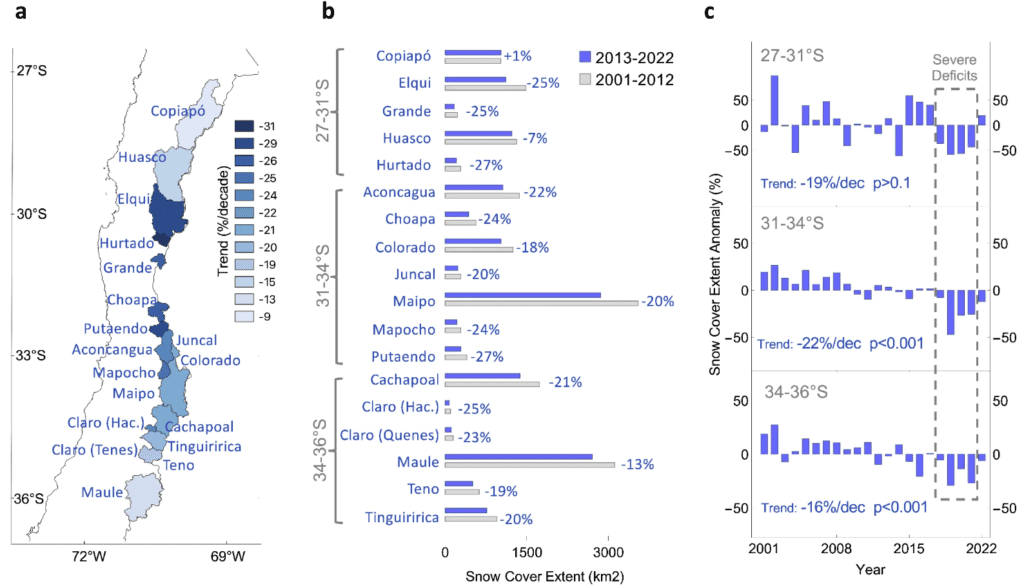
Abstract: Seasonal snow in the extratropical Andes is a primary water source for major rivers supplying water for drinking, agriculture, and hydroelectric power in Central Chile. Here, we used estimates from the Moderate Resolution Imaging Spectroradiometer (MODIS) to analyze changes in snow cover extent over the period 2001–2022 in a total of 18 watersheds spanning approximately 1,100 km across the Chilean Andes (27–36°S). We found that the annual snow cover extent is receding in the watersheds analyzed at an average pace of approximately 19% per decade. These alarming trends have impacted meltwater runoff, resulting in historically low river streamflows during the dry season. We examined streamflow records dating back to the early 1980s for 10 major rivers within our study area. Further comparisons with large-scale climate modes suggest that the detected decreasing trends in snow cover extent are likely driven by the poleward migration of the westerly winds associated with a positive trend in the Southern Annular Mode (SAM).
Fig. 1. The snow cover extent is rapidly declining in the extratropical Andes. (a) Trend in the annual snow cover extent of 18 watersheds in Central Chile (from latitude 27°S to 36°S), computed from MODIS-derived estimates over the period 2001–2022. (b) Changes in snow cover extent from 2001–2012 to 2013–2022 in 18 watersheds in Central Chile. (c) Annual snow cover extent relative to the 2001–2020 mean. The watersheds in (a) were grouped into three regions based on latitude: 27–31°S, 31–34°S, and 34–36°S.
Our new paper, “The water balance representation in Urban-PLUMBER land surface models“, is published in Journal of Advances in Modeling Earth Systems (IF: 4.4).
Authors: H. J. Jongen, M. Lipson, A. J. Teuling, S. Grimmond, J.-J. Baik, M. Best, M. Demuzere, K. Fortuniak, Y. Huang, M. G. De Kauwe, R. Li, J. McNorton, N. Meili, K. Oleson, S.-B. Park, T. Sun, A. Tsiringakis, M. Varentsov, C. Wang, Z.-H. Wang, G. J. Steeneveld
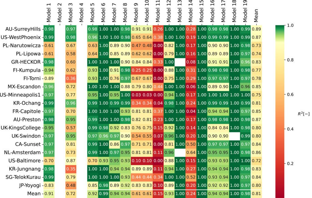
Abstract: Urban Land Surface Models (ULSMs) simulate energy and water exchanges between the urban surface and atmosphere. However, earlier systematic ULSM comparison projects assessed the energy balance but ignored the water balance, which is coupled to the energy balance. Here, we analyze the water balance representation in 19 ULSMs participating in the Urban-PLUMBER project using results for 20 sites spread across a range of climates and urban form characteristics. As observations for most water fluxes are unavailable, we examine the water balance closure, flux timing, and magnitude with a score derived from seven indicators expecting better scoring models to capture the latent heat flux more accurately. We find that the water budget is only closed in 57% of the model-site combinations assuming closure when annual total incoming fluxes (precipitation and irrigation) are within 3% of the outgoing (all other) fluxes. Results show the timing is better captured than magnitude. No ULSM has passed all water balance indicators for any site. Models passing more indicators do not capture the latent heat flux more accurately refuting our hypothesis. While output reporting inconsistencies may have negatively affected model performance, our results indicate models could be improved by explicitly verifying water balance closure and revising runoff parameterizations. By expanding ULSM evaluation to the water balance and related to latent heat flux performance, we demonstrate the benefits of evaluating processes with direct feedback mechanisms to the processes of interest.
Figure 8. Coefficient of determination (R2) between (half-)hourly explicit and implicit water storage change by model and site. Green indicates the 0.9 IS,t threshold. Missing results are shown as white (i.e., cannot calculate explicit or implicit water storage change).
Authors: Sarah Feron, Raúl R. Cordero, Alessandro Damiani, Shelley MacDonell, Jaime Pizarro, Katerina Goubanova, Raúl Valenzuela, Chenghao Wang, Lena Rester, Anne Beaulieu
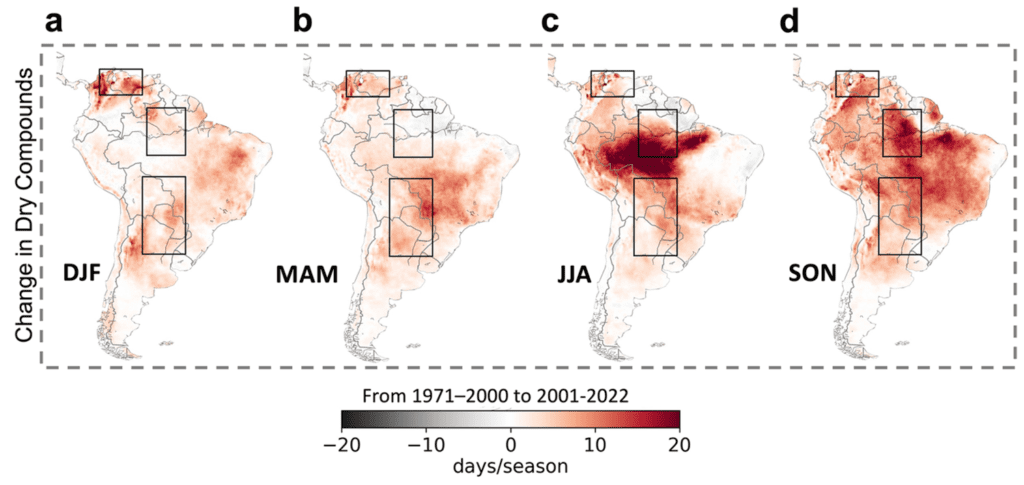
Abstract: South America is experiencing severe impacts from climate change. Although the warming of the subcontinent closely follows the global path, the rise of temperatures has been more pronounced in some regions, which have also seen a parallel increment in the occurrence of droughts and weather conditions associated with enhanced fire risk. Here, we use reanalysis datasets to analyze the progression of the concurring warm, dry, and high fire risk conditions (i.e., dry compounds) since 1971. We show that the frequency of these compound extremes has surged in key South American regions including the northern Amazon, which have seen a 3-fold increase in the number of days per year with extreme fire weather conditions (including high temperatures, dryness, and low humidity). Our results also suggest that the surface temperature of the tropical Pacific Ocean modulates the interannual variability of dry compounds in South America. While El Niño enhances the fire risk in the northern Amazon, dry extremes in the Gran Chaco region appear to be more responsive to La Niña.
Fig. 3: Dry compound extremes exhibit different regional and seasonal trends. Changes from 1971–2000 to 2001–2022 in the number of days per season with concurring warm, dry, and flammable conditions (i.e., dry compound days). The following meteorological seasons were considered: (a) December-January-February (DJF), (b) March-April-May (MAM), (c) June-July-August (JJA), and (d) September-October- November (SON). The number of dry compound days per season was derived (see “Methods”) from daily estimates from the ERA5 dataset over the period 1971–2022.
Our new paper, “Unraveling the discrepancies between Eulerian and Lagrangian moisture tracking models in monsoon- and westerly-dominated basins of the Tibetan Plateau“, is published in Atmospheric Chemistry and Physics (IF: 5.2).
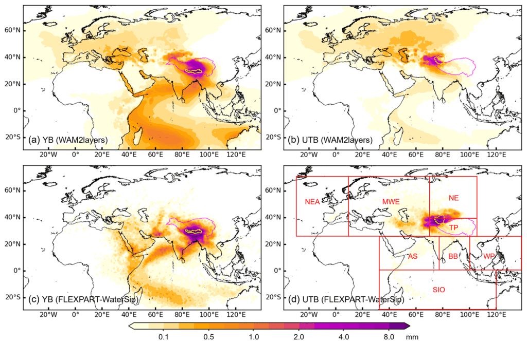
Abstract: Eulerian and Lagrangian numerical moisture tracking models, which are primarily used to quantify moisture contributions from global sources to specific regions, play a crucial role in hydrology and (paleo)climatology studies on the Tibetan Plateau (TP). Despite their widespread applications in the TP region, potential discrepancies in their moisture tracking results and their underlying causes remain unexplored. In this study, we compare the most widely used Eulerian and Lagrangian moisture tracking models over the TP, i.e., WAM2layers (the Water Accounting Model – 2 layers) and FLEXPART-WaterSip (the FLEXible PARTicle dispersion model coupled with the “WaterSip” moisture source diagnostic method), specifically focusing on a basin governed by the Indian summer monsoon (Yarlung Zangbo River basin, YB) and a westerly-dominated basin (upper Tarim River basin, UTB). Compared to the bias-corrected FLEXPART-WaterSip, WAM2layers generally estimates higher moisture contributions from westerly-dominated and distant sources but lower contributions from local recycling and nearby sources downwind of the westerlies. These differences become smaller with higher spatial and temporal resolutions of forcing data in WAM2layers. A notable advantage of WAM2layers over FLEXPART-WaterSip is its closer alignment of estimated moisture sources with actual evaporation, particularly in source regions with complex land–sea distributions. However, the evaporation biases in FLEXPART-WaterSip can be partly corrected through calibration with actual surface fluxes. For moisture tracking over the TP, we recommend using high-resolution forcing datasets, prioritizing temporal resolution over spatial resolution for WAM2layers, while for FLEXPART-WaterSip, we suggest applying bias corrections to optimize the filtering of precipitation particles and adjust evaporation estimates.
Figure 3. Spatial distributions of moisture contributions (equivalent water height over source regions; mm) to precipitation in July 2022 in the (a, c) YB and (b, d) UTB simulated by (a, b) WAM2layers and (c, d) FLEXPART-WaterSip. Purple lines represent the TP boundary, and yellow lines represent the boundaries of the two representative basins. Red boxes in (d) delineate the eight source regions: northeastern Atlantic (NEA), midwestern Eurasia (MWE), northern Eurasia (NE), TP, Arabian Sea (AS), Bay of Bengal (BB), western Pacific (WP), and southern Indian Ocean (SIO).
Our new paper, “Improving estimation of diurnal land surface temperatures by integrating weather modeling with satellite observations“, is published in Remote Sensing of Environment (IF: 11.1).
Authors: Wei Chen, Yuyu Zhou, Ulrike Passe, Tao Zhang, Chenghao Wang, Ghassem R. Asrar, Qi Li, Huidong Li
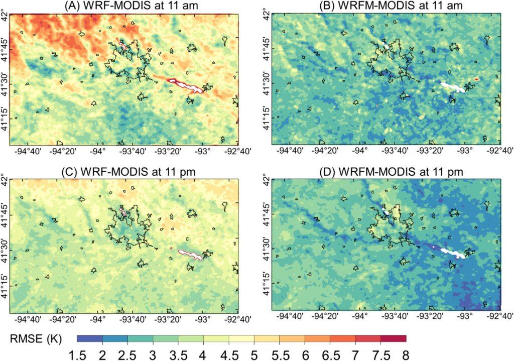
Abstract: Land surface temperature (LST) derived from satellite observations and weather modeling has been widely used for investigating Earth surface-atmosphere energy exchange and radiation budget. However, satellite-derived LST has a trade-off between spatial and temporal resolutions and missing observations caused by clouds, while there are limitations such as potential bias and expensive computation in model calibration and simulation for weather modeling. To mitigate those limitations, we proposed a WRFM framework to estimate LST at a spatial resolution of 1 km and temporal resolution of an hour by integrating the Weather Research and Forecasting (WRF) model and MODIS satellite data using the morphing technique. We tested the framework in eight counties, Iowa, USA, including urban and rural areas, to generate hourly LSTs from June 1st to August 31st, 2019, at a 1 km resolution. Upon evaluation with in-situ LST measurements, our WRFM framework has demonstrated its ability to capture hourly LSTs under both clear and cloudy conditions, with a root mean square error (RMSE) of 2.63 K and 3.75 K, respectively. Additionally, the assessment with satellite LST observations has shown that the WRFM framework can effectively reduce the bias magnitude in LST from the WRF simulation, resulting in a reduction of the average RMSE over the study area from 4.34 K (daytime) and 4.12 K (nighttime) to 2.89 K (daytime) and 2.75 K (nighttime), respectively, while still capturing the hourly patterns of LST. Overall, the WRFM is effective in integrating the complementary advantages of satellite observations and weather modeling and can generate LSTs with high spatiotemporal resolutions in areas with complex landscapes (e.g., urban).
Fig. 9. The RMSE between the WRF simulated (A&C) and WRFM generated (B&D) LSTs according to MODIS observed LSTs at 11 am and 11 pm, respectively. The boundary of urban areas was marked in black.
Yu Ding recently joined the Sustainable URban Futures (SURF) Lab as a Ph.D. student in Meteorology. Welcome!
Before coming to OU, Yu Ding completed her master’s degree in Hydrology and Water Resources at Hohai University, China. Her previous research focused on improving the accuracy of satellite precipitation data and integrating bias correction and machine learning algorithms to enhance data precision. Yu has an interest in utilizing remote sensing techniques and hydrological modeling.
Her Ph.D. research will focus on developing an integrated high-resolution pollutant dispersion model over complex terrain (e.g., urban environments).
Bohong Li recently joined the Sustainable URban Futures (SURF) Lab as a visiting M.Sc. student. Welcome!
Bohong Li is an M.Sc. student majoring in Atmospheric Science from the University of Hamburg. He finished his B.Sc. degree in meteorology in the University of Hamburg. In his bachelor thesis, he analyzed steep temperature drops using data from the Hamburg Weather Mast. Bohong’s research interests include urban climate and emission, atmospheric chemistry, urban heat island, as well as health risk and public health due to changing urban climate. During his visit, his research will focus on urban effects on precipitation.
Bohong’s personal interests include everything about Taylor Swift, sports and esports, gaming, photography, and watching series and movies.
Our new paper, “Methane dynamics altered by reservoir operations in a typical tributary of the Three Gorges Reservoir“, is published in Water Research (IF: 11.4).
Authors: Jia Liu, Fei Xue, Xiaojuan Guo, Zhengjian Yang, Manchun Kang, Min Chen, Daobin Ji, Defu Liu, Shangbin Xiao, and Chenghao Wang
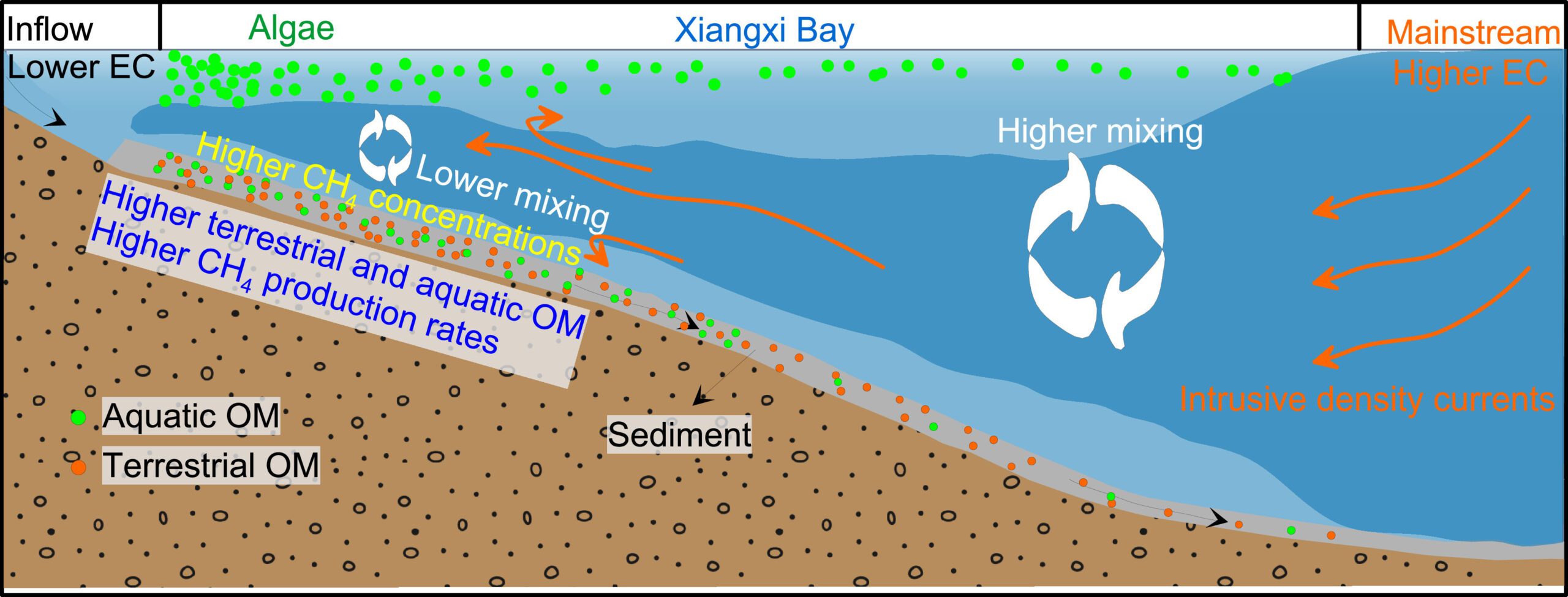
Abstract: Substantial nutrient inputs from reservoir impoundment typically increase sedimentation rate and primary production. This can greatly enhance methane (CH4) production, making reservoirs potentially significant sources of atmospheric CH4. Consequently, elucidating CH4 emissions from reservoirs is crucial for assessing their role in the global methane budget. Reservoir operations can also influence hydrodynamic and biogeochemical processes, potentially leading to pronounced spatiotemporal heterogeneity, especially in reservoirs with complex tributaries, such as the Three Gorges Reservoir (TGR). Although several studies have investigated the spatial and temporal variations in CH4 emissions in the TGR and its tributaries, considerable uncertainties remain regarding the impact of reservoir operations on CH4 dynamics. These uncertainties primarily arise from the limited spatial and temporal resolutions of previous measurements and the complex underlying mechanisms of CH4 dynamics in reservoirs. In this study, we employed a fast-response automated gas equilibrator to measure the spatial distribution and seasonal variations of dissolved CH4 concentrations in XXB, a representative area significantly impacted by TGR operations and known for severe algal blooms. Additionally, we measured CH4 production rates in sediments and diffusive CH4 flux in the surface water. Our multiple campaigns suggest substantial spatial and temporal variability in CH4 concentrations across XXB. Specifically, dissolved CH4 concentrations were generally higher upstream than downstream and exhibited a vertical stratification, with greater concentrations in bottom water compared to surface water. The peak dissolved CH4 concentration was observed in May during the drained period. Our results suggest that the interplay between aquatic organic matter, which promotes CH4 production, and the dilution process caused by intrusion flows from the mainstream primarily drives this spatiotemporal variability. Importantly, our study indicates the feasibility of using strategic reservoir operations to regulate these factors and mitigate CH4 emissions. This eco-environmental approach could also be a pivotal management strategy to reduce greenhouse gas emissions from other reservoirs.
Fig. 6. Conceptual diagram of CH4 dynamics in Xiangxi Bay under the operations of the Three Gorges Reservoir. The light blue area represents inflow from upstream of XXR, while the dark blue area represents flow from the mainstream. Orange and green circles along the riverbed represent terrestrial and aquatic OM, respectively. Solid green circles near the water surface represent algae.
Our new paper, “A modeling framework to assess fenceline monitoring and self-reported upset emissions of benzene from multiple oil refineries in Texas“, is published in Atmospheric Environment X (IF: 3.8).
Authors: Qi Li, Lauren Padilla, Tammy Thompson, Shuolin Xiao, Elizabeth Mohr, Xiaohe Zhou, Nino Kacharava, Yuanfeng Cui, and Chenghao Wang
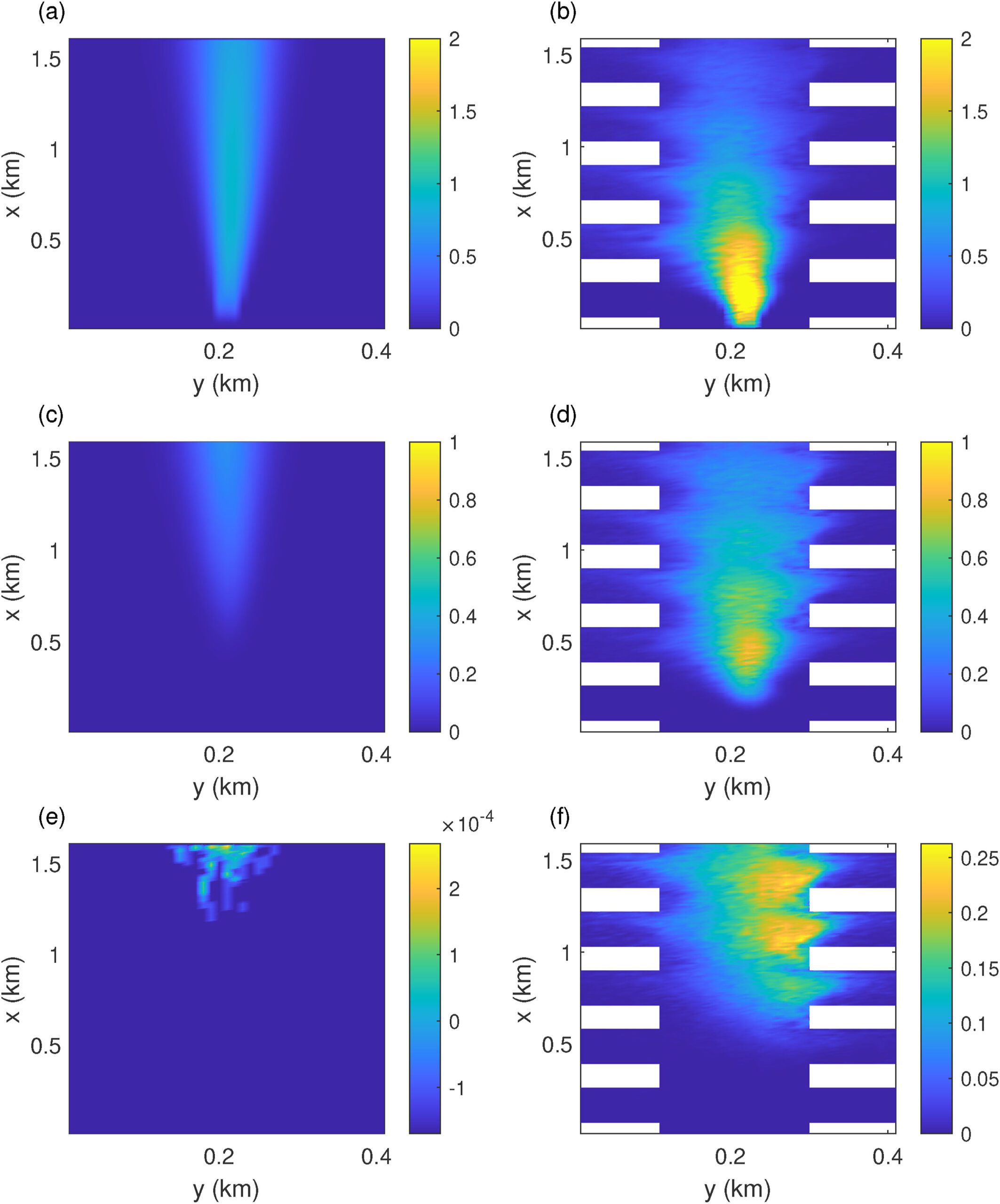
Abstract: Benzene as one type of hazardous air pollutants (HAPs) is produced by industrial production processes and/or emitted during upset events caused by man-made or natural accidents. Although upset emissions of benzene can be a significant contributor to the total emission, it is still challenging to quantify. This study first develops a fast modeling framework using obstacle-resolving computational fluid dynamics modeling to compare the modeled within-facility-scale passive pollutant dispersion with the observed levels based on self-reported emissions for fourteen facilities in Texas, United States. Results of numerical simulations demonstrate that neglecting the obstacle effect can underpredict (overpredict) the near-(far-)field concentrations for a low source. For a source located above obstacles, underprediction occurs at all distances. The diagnostic framework is applied to 107 self-reported upset emission events for fourteen petroleum refineries in Texas from year 2019–2022. Considering different metrics across all events, it can be concluded that the modeled concentrations based on self-reported emissions likely underpredict the observed concentration increments. Depending on the possible source height, the median factor of underprediction ranges from 3 to 95 based on the average-plume metric. The agreement between model and observation is better for events characterized by high emission amounts and rates, which also correspond to high observed concentration increments. Overall, the research highlights the importance of considering obstacles and demonstrates the potential application of the current approach as an efficient diagnostic method for self-reported upset emissions using fenceline observations of HAPs.
Fig. 2. Normalized concentrations for cases without and with obstacles for horizontal plane at z = 2 m. The wind direction is zero degree, the obstacle geometry is sparse-low. The obstacles, i.e., the “white-bars” are 100 m × 100 m and the gap between, d, is 200 m in this example. The planar location of the source is indicated by the blue star in Fig. 1a; the top, middle, to bottom rows show cases with source heights corresponding to low, medium, and high as indicated in Fig. 1b. (a), (c), (e): C’LES for cases without obstacles with source heights zs low, medium and high. (b), (d), (f): C’LES for case with sparse-low obstacles with source heights zs low, medium and high.